

I’ve thought a lot about this connected scatterplot from the Washington Post’s Philip Bump over the previous few months.

I’m not interested in the graph because the data are particularly interesting or I care so much about President Biden’s approval ratings, but instead because it created a bit of a stir in the data visualization Twitter community. Is it bad because many people don’t know how to read a connected scatterplot? Is it good because it layers the two series together?
But, in early January, I saw this tweet from Len Kiefer where he placed two line charts on the left side of the graphic and a connected scatterplot on the right side of the graphic. What a solution! Let people see the two time series independently in a graph form they are familiar with and then also put the two together in the connected scatterplot format!
How would it work with Philip’s chart? I grabbed the data from the two sources listed in his column (FiveThirtyEight and Energy Information Administration housed at the St. Louis FRED tool) and did some quick tabs to get the data close (though not exact) to what he showed. I popped them into Tableau, made two line charts and a connected scatterplot (thank you, Information Lab for the Tableau tutorial), and aligned them in a way similar to Len’s graphic. This is what I end up with.
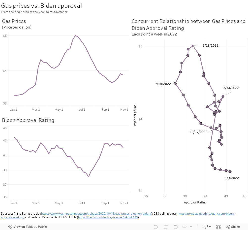
I gotta say, that’s pretty darn cool. You can see the rise and fall of gas prices over the year in the top graph and the paired fall and rise of Biden’s approval ratings in the bottom graph. I’m not sold on my title for the connected scatterplot (“Concurrent Relationship between Gas Prices and Biden Approval Rating”) but wanted to give it a title rather than leaving that space blank.
I think there is one more step I can apply to further clarify the visual, which is to modify the colors. I color the lines for the first half of the year—when gas prices were heading up and approval ratings down—in orange, and the second half of the year in blue. In this format, I think the pieces hold together a little bit better and the entire graphic becomes clearer.
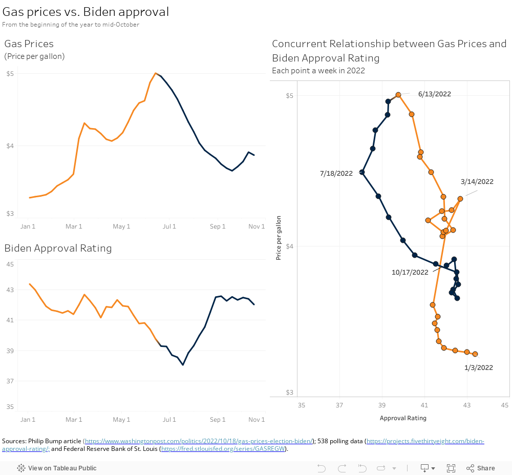
What do you think? A useful technique? Personally, this might be my new way forward when it comes to connected scatterplots.
UPDATE: Albert Rapp has created a template in R with open source code available on his Github repo.


Hi Jon, I love that the colour encoding here adds immediate insight to the relationship of the variables and would accommodate different turning/threshold points (eg you could have more than the two time periods differentiated, or over a longer time series you could colour-coordinate quarters/seasons of the year etc).
Where the data points cluster (as in the blue end of the connected scatterplot and in the orange segment around March to May, what do you think about making the encoding work harder here to convey the direction of the line? For instance, you could use colour gradients to signal which data point occurs before the next one (either in the line itself or in the markers perhaps), or alternatively, gradations of weight of the line (eg starting from heaviest/thickest at 1/3/2022 and then becoming lighter/thinner through to the 6/13/2022 point, and then the reverse treatment heading to the end of the blue segment)?
I’m coming at this from a graphic design perspective, rather than a coding one, so I don’t know how hard it would be to make this work, but hopefully you see what I’m getting at? I’m looking for a way to make it easy to follow the direction of the connected scatter plot where a line crosses over itself. Obviously it’s easy enough to hover over a data point online and discern the sequence, but for an offline/printed version of the chart, it would be good to have a clear way to discern which crossover happens first…no?
Hi Jane,
Thanks for your comment and I’m glad you like this approach. I agree that the two clusters (March and October) make it harder to pull out specific trends at those times. One could add color gradients–or even additional text annotations and arrows–at those time periods. In Tableau, creating those color gradients should be pretty easy to do.