

One of the encouraging trends in the data visualization space right now is the focus on accessibility. While the data visualization field has for too long focused solely on visual impairments—primarily red-green color vision deficiency or “color blindness”—there is more work and consideration around screen readers, alt text, sonification, and other ways to make data and data visualizations more accessible to broader audiences.
For me, data visualizations that don’t meet basic visual accessibility guidelines—colors that may not be accessible next to each other or insufficient contrast between pairs of colors—have become easier to spot. For example, this graph from Data For Progress popped up in my Twitter feed a few days ago and my immediate reaction was, “there is no way the text in those light blue bars is accessible.” A quick check at WebAIM, my favorite color contrast checker, confirmed that starting with the fifth bar (Gun control), the white-blue color combination was not accessible under the standard normal text WCAG recommendations. (Quick note: the way I test this is to open the Digital Color Meter on my Mac, put the cursor over the bar and click the SHIFT+CMD+C keyboard shortcut. This copies the HEX code to the clipboard, which I then paste into the box on the WebAIM website.)

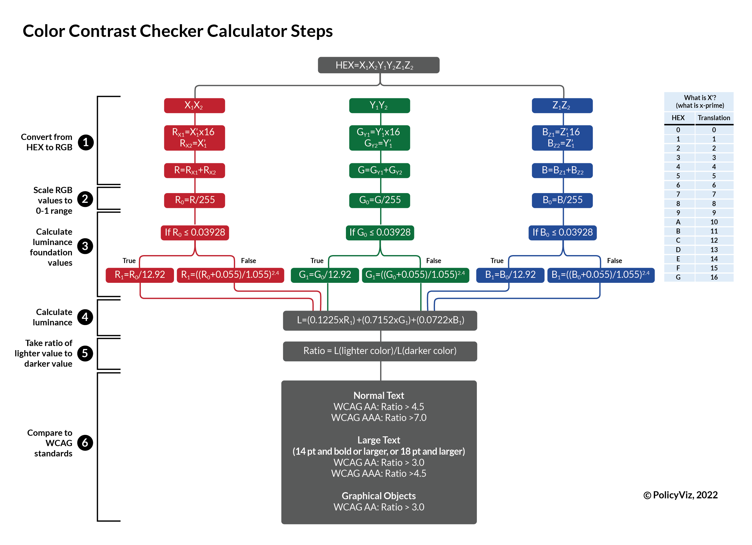
Instead of calculating the HEX code for each bar and typing it into the WebAIM tool—or any of the other tools I’ve collected—I thought I could create my own color contrast tool in Excel. I did so for two reasons: First, I wanted to be able to test multiple colors quickly. And second, it seemed like a good challenge. But maybe too good of a challenge. There are a lot of steps here, which the image below tries to summarize. In sum, I need to convert HEX codes to RGB codes, then calculate the luminance value for each color, and then compare the pairs.

I’ll walk through each of the six steps and the Excel calculations that need to happen to make it work. I also added a macro to my Excel file, which automatically colors the cell based on the HEX code in the cell. You can download my Excel file to use on your own.
- Convert the HEX code to RGB. Hex codes are six-digit hexadecimal numbers that represent colors. Each two-digit pair of the code represents a color, so I need to convert each element to decimal values. The value of each pair is converted to a decimal equivalent—0 to 0, 1 to 1,…, A to 10, B to 11, and so on, so it is then equivalent to each piece of the RGB color model. Thus, the first pair of the orange color HEX code #F58700, F5, will be equivalent to R in RGB. In this case, ‘F5’ converts to 15 for F and 5 for 5 (see the blue table towards the right in the above image). I multiply the first decimal value by 16 and add it to the second value: 15×16 + 8 = 240 + 5 = 245.
- This is a little complicated in Excel, and there are two steps. First, I use the MID() formula to pull out each individual value from the HEX code, generating six values in six separate cells. I also need to distinguish between letters and numbers. If the digit is a number, Excel will enter it into the cell as a character, so I also need to convert it to a number using the VALUE() function inside a long IF formula:
For the first digit, I use the following formula:
=IF(ISNUMBER(VALUE(MID($B2,D$1,1))), VALUE(MID($B2,D$1,1)), MID($B2,D$1,1))
Let’s work inside out: The MID($B2,D$1,1) function looks at the HEX code (in cell B2) and looks in cell D1 for the starting value (set equal to two—the first digit after the hashtag) and pulls out the number of digits specified in the last argument (one). The VALUE function will convert whatever the value is from the MID() function to a number.
The first part of the IF statement tests whether the value of the first digit—from the MID() function—is a number (checked by the ISNUMBER formula). If the evaluation in the first part of the IF formula is TRUE (it is a number), the second argument says to enter the value of that first digit in the cell (as a number). If the evaluation is FALSE—it is a character—then the IF formula says to just enter that letter in the cell.
With the extracted HEX values, I convert each value to its corresponding decimal equivalent. I use a VLOOKUP value using the little table on the right side in the image above, which is placed in cells AD2:AD18 in my Excel file. The VLOOKUP for the F value in the HEX code is:
=VLOOKUP(D2,$AD$2:$AE$18,2,0)×16.
Very simply, Excel looks at the first R value (“F”) and extracts the value in the second column of the lookup table, which is 15. These steps are repeated for each of the six HEX characters and then converted to single R, G, and B colors by summing the pairs together. These steps are repeated for each of the six HEX characters and then converted to single R, G, and B colors by summing the pairs together.
- Normalize each element in the RGB code to a 0-to-1 scale. We need to normalize each of the three RGB codes to a scale between 0 and 1. Because each is bounded between 0 and 255, we simply divide by 255. In our example of the R color for the #F58700 color, we get R0 = 245/255 = 0.961.
- This is easy in Excel—simply divide each of the three codes by 255.
- Calculate the RGB luminance foundation values. Now we get into some more complicated math. We are going to take our scaled RGB colors, R0, G0, and B0, and compare it to a fixed value of 0.03928. (I take the scalar values on faith here but am not completely sure where they come from.) If our scaled values are less than or equal to the 0.03928 scalar, we divide it by 12.92; otherwise, we use an even more complicated formula: ((R0+0.055)/1.055)2.4 (again, not 100% where this comes from). In our example, R0 = 0.961, which is greater than 0.03928, so we end up with ((0.961+0.055)/1.055)2.4 = 0.931.
- This isn’t terribly difficult in Excel, but it does require some careful typing. We use an IF statement to check the 0.03928 inequality and each of the other arguments tells Excel what to do depending on the inequality:
=IF(V2<=0.03928, V2/12.92, ((V2+0.055)/1.055)2.4)
If the scaled value is less than 0.03928, we simply divide by 12.92; otherwise, we use the more complicated equation.
- Calculate the luminance value. We use the relatively simple formula here: L = (0.2126 × R1) + (0.7152 × G1) + (0.0722 × B1), which, for our example, becomes L = (0.2126 × 0.961) + (0.7152 × 0.529) + (0.0722 × 0.000) = 0.367.
- Take the ratio of the lighter color to the darker color. The WebAIM tool calls these the “Foreground” and “Background” colors, but the math requires figuring out which color is lighter than the other—that is, the larger Luminance value (plus 0.05) divided by the smaller Luminance value (plus 0.05) = (Llight + 0.05)/(Ldark + 0.05).
- Again, a little formula work makes this easy. I use a MAX and MIN function to determine which of the two-color pairs I want to put in the numerator and denominator. In other words, =(MAX(colorA, colorB)+0.05)/(MIN(colorA, colorB)+0.05).
- Compare the ratio to the WCAG standards. After all this math is complete, we can simply take the final ratio and compare it to the WCAG cutoffs shown in the image above.
- This is a simple set of IF statements in Excel with some added conditional formatting to highlight the PASS/FAIL results.
Let’s put this through an example by placing orange text (HEX code #F58700) on a blue background (#264B96).
| Orange (#F58700) | ||||||
| HEX code | F | 5 | 8 | 7 | 0 | 0 |
| Decimal | 15×16 | 5 | 8×16 | 7 | 0×16 | 0 |
| R1,R2,… | 240 | 5 | 128 | 7 | 0 | 0 |
| RGB | 245 | 135 | 0 | |||
| Scaled | 245/255 = 0.961 | 135/255 = 0.528 | 0/255 = 0 | |||
| Check: ≤ 0.03928? | No | No | Yes | |||
| Luminance Foundation | (0.961+0.055)/1.055)2.4 = 0.913 | (0.528+0.055)/1.055)2.4 = 0.242 | 0/12.92 = 0 | |||
| Luminance | = 0.2126×0.913 + 0.7152×0.242 + 0.0722×0 = 0.367 | |||||
| OBlue (#264B96) | ||||||
| HEX code | 2 | 6 | 4 | B | 9 | 6 |
| Decimal | 2×16 | 6 | 4×16 | 11 | 9×16 | 6 |
| R1,R2,… | 32 | 6 | 64 | 11 | 144 | 6 |
| RGB | 38 | 75 | 150 | |||
| Scaled | 38/255 = 0.149 | 72/255 = 0.294 | 150/255 = 0.588 | |||
| Check: ≤ 0.03928? | No | No | No | |||
| Luminance Foundation | (0.149+0.055)/1.055)2.4 = 0.070 | (0.294+0.055)/1.055)2.4 = 0.305 | (0.588+0.055)/1.055)2.4 = 0.076 | |||
| Luminance | = 0.2126×0.019 + 0.7152×0.070 + 0.0722×0.305 = 0.076 | |||||
| | Orange (#F58700) | Blue (#264B96) |
| Luminance | 0.367 | 0.076 |
| Max (lighter) | 0.367 | |
| Min (darker) | 0.076 | |
| Ratio | (0.367 + 0.05)/(0.076 + 0.05) = 3.30 | |
| | Cutoff for Pass | Luminance Ratio | Pass/Fail |
| Normal Text | |||
| WCAG AA | 4.5 | 3.30 | FAIL |
| WCAG AAA | 7.0 | 3.30 | FAIL |
| Large Text (14 pt and bold or larger, or 18 pt and larger) | |||
| WCAG AA | 3.0 | 3.30 | PASS |
| WCAG AAA | 4.5 | 3.30 | FAIL |
| Graphical Objects | |||
| WCAG AA | 3.0 | 3.30 | PASS |
What about the Data For Progress graph that kicked this whole thing off? Well, turns out that doing multiple comparisons between the bar color and the white text is easier to do with this Excel calculator than the WebAIM tool because it’s a simple task of pasting in the HEX codes rather than separately copying-and-pasting each code into the browser. The screenshot below shows all the columns necessary to get this to work, but you can see that only the first five blue colors pass the WCAG AA Normal Text cutoff of a luminance ratio of at least 4.5.

Wrap Up
As I mentioned, there are many good color contrast tools available for you to use online, usually for free. And while most of them make it easy to tweak your colors with a slider or color picker tool, I don’t think any of them let you do a batch comparison quite like this. Please feel free to download my Excel file (be sure to Enable Macros the cell-color macro will run) and use it, tweak it, and share it.
Did you like this post? Did you know that you could have seen it earlier if you signed up for my newsletter or my Winno community? Sign up now to get great dataviz-related stuff!


You can streamline and simplify some of the formulas. Convert the hex color to normalized RGB values using:
=HEX2DEC(LEFT(TEXT(A2,”000000″),2))/255
=HEX2DEC(MID(TEXT(A2,”000000″),3,2))/255
=HEX2DEC(RIGHT(TEXT(A2,”000000″),2))/255