How to define a map’s bins to visualize your data

How many maps have you seen and not thought twice about how the data are plotted? Has the author carefully considered the colors assigned to the geographic units? Are the data placed into reasonably sized bins or groups? How were those bins chosen? Too often, we let our software tools make these decisions for us. But when we take greater control of these choices, we can make conscious, purposeful decisions that help readers reach conclusions and gain insights from the data.

With any map that visualizes data, we can make decisions about some primary characteristics, including the map projection, colors, and bin number and width. Here, I focus on how bins are presented in a map’s legend.

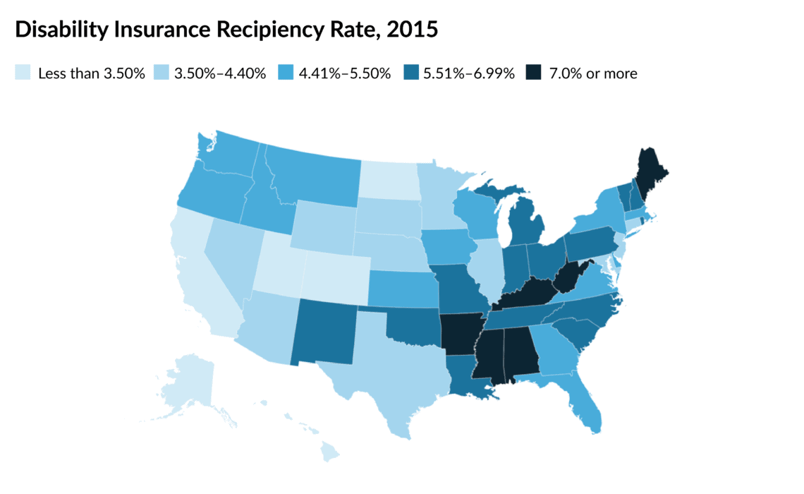
Let’s start with this map of the geographic dispersion in the Disability Insurance (DI) recipiency rate—that is, the number of people receiving DI benefits as a share of the 18-to-65 population. The data are placed into five groups. You can quickly see, for example, that Arkansas, Maine, West Virginia, and other dark-blue states have the highest recipiency rates.

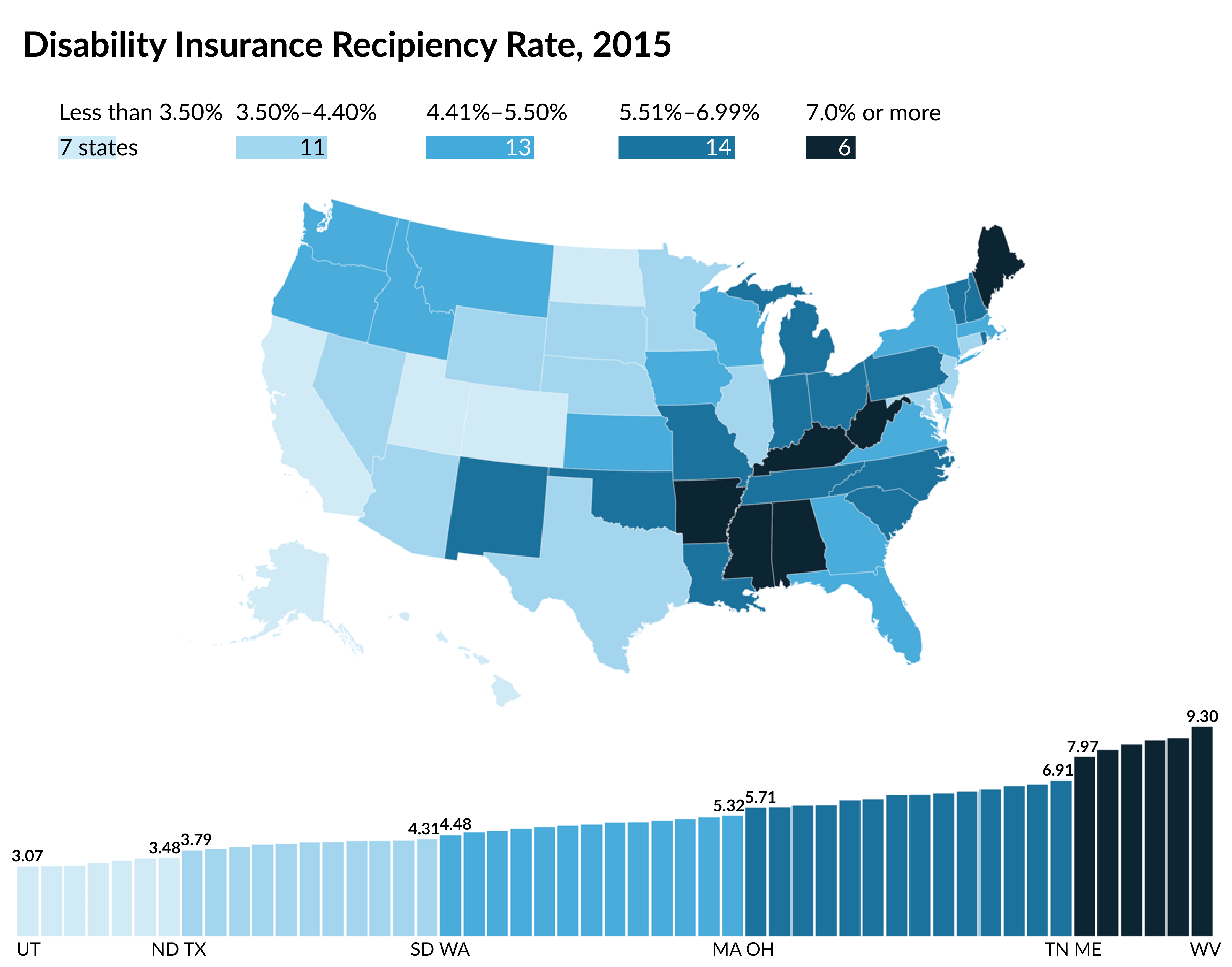
Placing the data into these categories results in an aggregation problem. We don’t know, for example, how different Arkansas, Maine, and West Virginia are from each other because they are grouped together. If we plot the same map but include a column chart, we can more easily see the differences in the values. Some visible jumps appear in the data, which can help define the bins.

You may also notice that the definition of the breaks in the legend are arbitrary. Look at the top bin: the recipiency rate jumps from 6.91 percent in Tennessee to 7.97 percent in Maine. Why then is the bin for the fifth group “7.0 percent or more”? It’s true, but it could have just as easily started at 7.5 percent or even 7.9 percent.

In fact, the legend for this map can be defined in multiple ways.

1. Instead of two decimal places, the legend could have used just one decimal place, but that still leaves us with arbitrary bins, and it isn’t clear if a value of 7.0 percent, for example, is in the fourth or fifth group.

1a. One possible solution—and something we have documented in the Urban Institute style guide—is to explicitly note which bins are inclusive or exclusive of the upper and lower bounds.

2. Another alternative would be to define the bins based on the actual data values.

This has the advantage of more clearly showing the data. For example, we can more clearly see the gap between 6.91 percent and 7.97 percent.

And yet, this legend may look odd. If you’re unfamiliar with the data, you may think, “What happened to the data between 6.91 percent and 7.97 percent?”

3. Alternatively, we could create a legend that includes these “gap” bins:

Although accurate and comprehensive, this legend feels busy and obscures the five original bins by adding the four nondata bins that connect the groups.

I’m not sure there is a perfect solution, but this map illustrates the variety of issues to consider, including the level of precision (i.e., the number of decimal places), the number of bins, and the smoothness of the data (i.e., if the data show no visible jumps, round-numbered bins may be fine).

In this example—and, I suspect, in many maps you see—I find it most helpful to define the bins based on the data and show the number of states in each.

In the map below, I’ve added a bar chart to serve as the legend where the length of the bars denote the number of states in each bin. This way, you can quickly see how the bins are defined and the number of observations in each.

Maps are a great way to show geographic data, but we should carefully consider our data and design decisions to help audiences understand the information we are trying to convey.

This post was originally published on the Urban Institute’s blog, Urban Wire on January 12, 2018.