Creating a Heatmap Legend in Excel

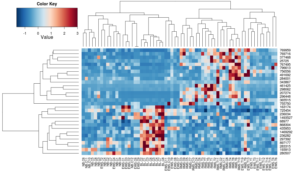
Someone recently asked me how to create a legend for a heatmap in Excel. In R, adding a legend is part of the package (the image below from a thread on StackOverflow), so it’s pretty easy to do. Building a heatmap legend in Excel is not that difficult and uses the same Conditional Formatting approach that is used to create the basic heatmap.

Step 1. Create the Heatmap

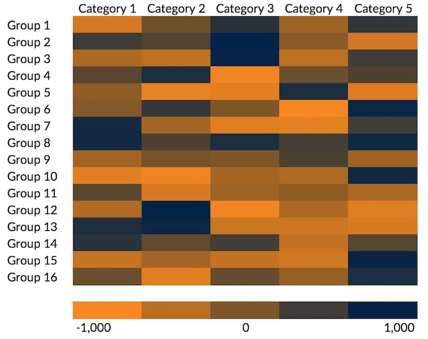
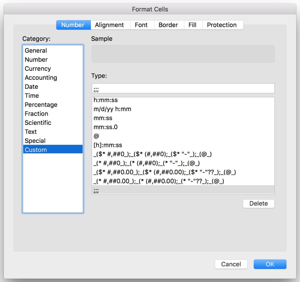
I’ve described this technique in a couple of posts already (here and here), so here’s a quick review: First, select the data and use the Color Scales option in the Conditional Formatting menu. To hide the numbers, select the data and in the Custom section of the Format Numbers menu, insert three semicolons (;;;) into the Type box.

Step 2. Create the Legend

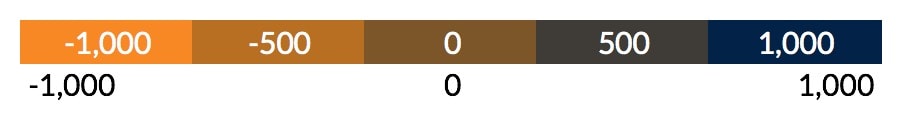
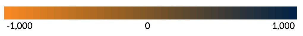
You need to understand your data, so in this version, I set the ends of the legend at the minimum (-1,000) and maximum (1,000) of the data set. I now create a new row with the far-left cell equal to that minimum and the far-right cell equal to the maximum. I use a simple step (+500) to insert numbers to the three cells in between. I then apply the same Conditional Formatting Color Scales to this row, hide the numbers, and put add the minimum, maximum, and center (0) numbers below the legend.

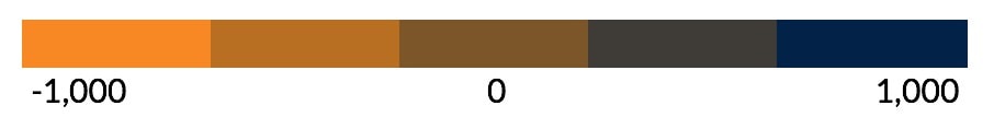
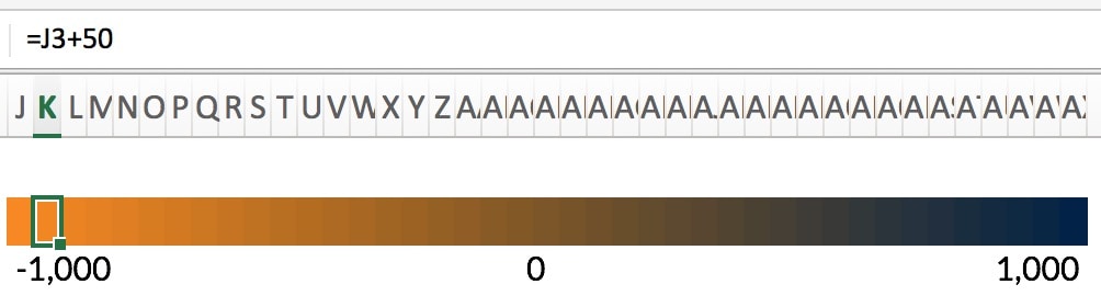
Alternatively, if you want a legend that has a more detailed ramp, you can do so by using more cells. In this version, I use 41 cells and reduced the width of each column to 9 pixels each. I calculate the slope to tick up by 50, instead of 500 in the first version. I again apply the Color Scales from Conditional Formatting and hide the numbers.

If I wanted to put the heatmap and this legend together in a single document, I might save both separately as images and then piece them together (maybe even as simply as using PowerPoint).